This is the first part of a series of posts on learnings from implementing toy flow matching experiments. The goal is to share practical insights as a way for me to consolidate my understanding, and hopefully be useful to anyone getting their hands dirty with flow matching for the first time.

Brief Overview of Flow Matching

Flow matching (Lipman et al., 2022) is a simulation-free generative modeling framework. The core idea: learn a velocity field $v_\theta(x_t, t)$ that transports samples from a simple source $p_0$ (a Gaussian) to the data distribution $p_1$.

Training. Given a pair $(x_0, x_1)$ with $x_0 \sim p_0$ and $x_1 \sim p_1$, form the linear interpolant $x_t = (1-t)\,x_0 + t\,x_1$ and regress the target velocity $\dot{x}_t = x_1 - x_0$ with MSE.

Sampling. Integrate $\dot{x} = v_\theta(x, t)$ from $t=0$ to $t=1$, starting from $x_0 \sim p_0$.

That’s essentially it. The elegance is that training never requires simulating the ODE — you just sample random $(x_0, x_1, t)$ triplets and fit the velocity. For a thorough treatment see the original paper, Flow Matching for Generative Modeling (Lipman et al., 2022).

The experiments below were done on two settings: a 2D two-moons dataset and MNIST. The code for all experiments is available in the flow-matching repository.

---

1. Base Noise Distribution: Variance Matters

The source distribution $p_0 = \mathcal{N}(\mu, \sigma^2 I)$ is a design choice, and it has a real effect on sample quality.

Intuitively, smaller $\sigma$ means shorter, nearly straight training trajectories that are easy to fit. But it also means noise samples cluster tightly together, which limits the diversity of generated outputs. Larger $\sigma$ gives the model more room to explore the space but produces longer, noisier paths that are harder to regress accurately.

In the MNIST experiments I swept $\sigma$ across an order of magnitude and found a clear pattern: training loss decreases monotonically as $\sigma$ shrinks, but sample quality degrades at the extremes in both directions.

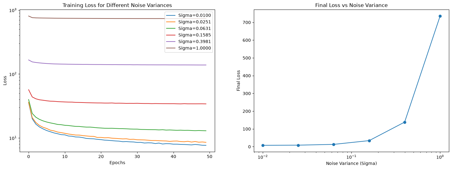
The sweet spot in my experiments was around $\sigma \approx 0.05$–$0.1$. At $\sigma = 0.01$ the model fits the training distribution nearly perfectly but generates samples with little variety, essentially memorizing a tight cluster. At $\sigma = 1.0$ the paths are so noisy that the model struggles to converge at all. The right value will depend on your dataset and model capacity, but defaulting to $\sigma = 1$ (standard Gaussian) is likely suboptimal for structured data like images.

---

2. ODE Solver: The Midpoint Method Pays Off

Sampling requires integrating the learned ODE from $t=0$ to $t=1$. The simplest choice is the Euler method, which takes $n$ steps of size $1/n$:

\[x_{t + \Delta t} = x_t + \Delta t \cdot v_\theta(x_t, t)\]

A better alternative is the midpoint method, which evaluates the velocity at the midpoint of each step:

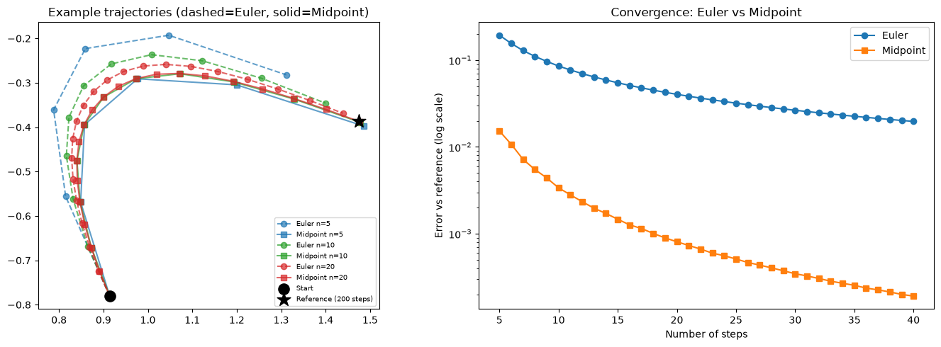
\[x_{t + \Delta t} = x_t + \Delta t \cdot v_\theta\!\left(x_t + \tfrac{\Delta t}{2} v_\theta(x_t, t),\; t + \tfrac{\Delta t}{2}\right)\]

This costs 2 network evaluations per step instead of 1, but the accuracy improvement is dramatic. In the 2D experiments, achieving similar endpoint error required roughly 40 Euler steps versus only 5 midpoint steps, an 8× reduction in the number of steps for the same effective cost per step.

In code, the midpoint step slots in cleanly:

def step(self, x_t: Tensor, t_start: Tensor, t_end: Tensor) -> Tensor:
    t_start = t_start.view(1, 1).expand(x_t.shape[0], 1)
    dt = t_end - t_start
    return x_t + dt * self(
        t=t_start + dt / 2,
        x_t=x_t + self(x_t=x_t, t=t_start) * dt / 2
    )

If you’re doing any FM inference and haven’t switched from Euler, this is a free win.

---

3. Optimal Transport Coupling

By default, training pairs each noise sample $x_0$ with a random data sample $x_1$, as you would get by simply shuffling a batch. The resulting interpolant trajectories $x_t$ can cross each other at arbitrary angles, and the velocity field has to be consistent with all of them simultaneously. This creates a harder learning problem.

Optimal transport (OT) coupling fixes this by solving a matching problem: given a batch of noise samples and a batch of data samples, find the assignment that minimizes total squared distance. In practice, this is just a linear sum assignment solved with scipy:

from scipy.optimize import linear_sum_assignment
from scipy.spatial import distance

cost = distance.cdist(x_0.numpy(), x_1.numpy())
row_ind, col_ind = linear_sum_assignment(cost)
x_0, x_1 = x_0[row_ind], x_1[col_ind]

The result is that each $x_0$ gets paired with the nearest (in batch) $x_1$, producing shorter, more parallel trajectories.

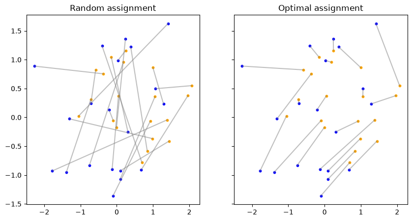
On the left, random coupling produces crossing trajectories. On the right, OT coupling produces much more parallel paths that are easier to regress. In the 2D experiments, OT training also converged to a lower final loss and did so faster. The downside is the added per-step cost of solving the assignment problem, which scales as $O(n^3)$. This is fine for moderate batch sizes, but something to watch at scale.

---

4. Class Conditional Flow Matching

On MNIST, conditioning on the class label lets us generate digits from a specific class at sampling time. It also improves sample quality in general, since the model doesn’t have to explain all ten classes with a single velocity field.

Samples generated with unconditioned FM:

Samples generated with class-conditioned FM:

I experimented with three different ways to inject class information.

Approach 1: Concatenating a compact class embedding

The most straightforward approach: learn a small $d$-dimensional embedding per class and concatenate it with $x_t$ and $t$ as input to the network.

class CondFlow(nn.Module):
    def __init__(self, dim: int = 784, h: int = 64, c_dim: int = 2):
        super().__init__()
        self.class_emb = nn.Embedding(10, c_dim)
        self.encoder = nn.Sequential(
            nn.Linear(dim + c_dim + 1, h),
            nn.ReLU(),
            nn.Linear(h, h),
        )
        self.decoder = nn.Sequential(
            nn.Linear(h, h),
            nn.ReLU(),
            nn.Linear(h, dim),
        )

    def forward(self, t: Tensor, c: Tensor, x_t: Tensor) -> Tensor:
        c_emb = self.class_emb(c)
        inp = torch.cat((x_t, c_emb, t), 1)
        z = self.encoder(inp)
        return self.decoder(z)

This works well. The class embedding is compact (just c_dim extra input dimensions), and the network has full flexibility to use it however it wants. At sampling time, fix the class label and integrate as usual.

Approach 2: Additive image-domain embedding

A variation I tried: instead of a compact latent embedding, give each class a full 784-dimensional prototype $e_c$ that gets added to $x_t$ in pixel space before encoding.

class CondFlow(nn.Module):
    def __init__(self, dim: int = 784, h: int = 64):
        super().__init__()
        self.class_emb = nn.Embedding(10, dim)  # 784-dim per class
        ...

    def forward(self, t: Tensor, c: Tensor, x_t: Tensor) -> Tensor:
        c_emb = self.class_emb(c)
        inp = torch.cat((x_t + c_emb, t), 1)
        z = self.encoder(inp)
        return self.decoder(z)

The original motivation was interpretability: since each $e_c$ lives in the same 784-dimensional pixel space as the images, you could visualize it as a 28×28 image and inspect what the model learned as a class prototype.

Samples generated from conditioned FM:

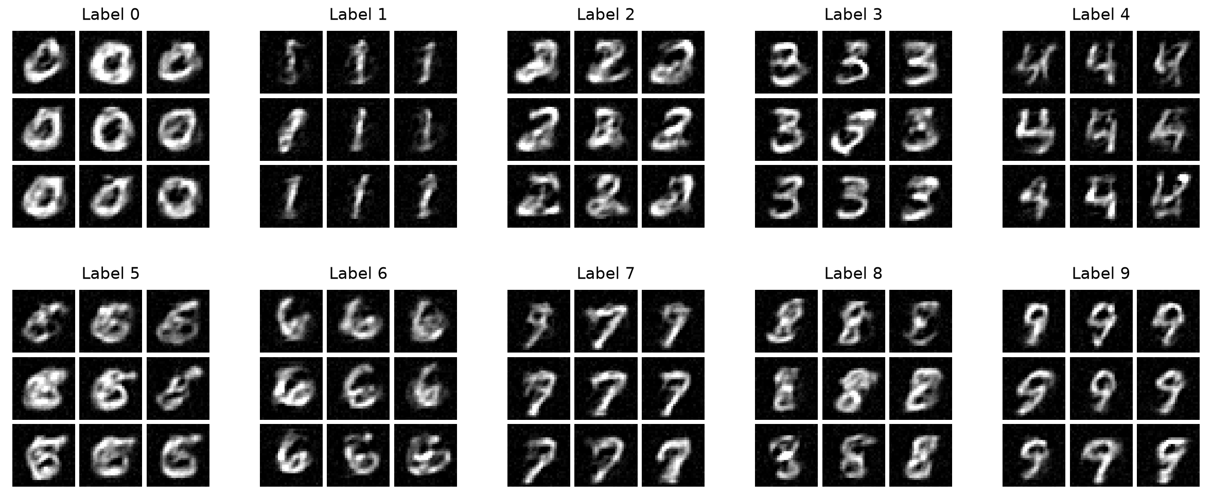
In practice, however, the learned embeddings don’t look like digits at all.

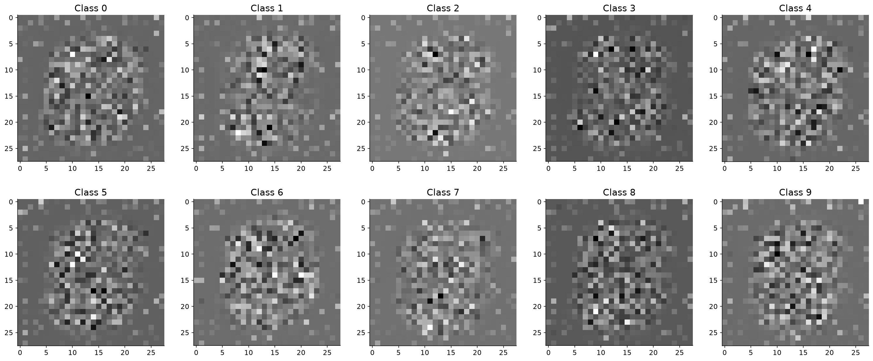
They’re not noise either; they have some structure, but there’s no visual correspondence to the class they’re supposed to represent. This makes sense in hindsight: the embeddings are optimized to minimize the flow matching loss, not to be interpretable to a human. The gradient signal pushes each $e_c$ toward whatever shift of $x_t$ makes the velocity regression easiest, which has no reason to align with what a digit looks like.

The takeaway is that placing an embedding in a semantically meaningful space (pixel space) doesn’t make it semantically meaningful. If interpretability is the goal, you need to add an explicit objective for it.

Approach 3: Conditioning on the base distribution

Both approaches above inject class information into the velocity field. There’s a different angle: condition on the source distribution instead of the velocity field. Concretely, learn a class-specific mean $\mu_c$ for $p_0$ and sample $x_0 \sim \mathcal{N}(\mu_c, \sigma^2 I)$ at training and inference time, while keeping the velocity field itself unconditional.

class CondBaseFlow(nn.Module):
    def __init__(self, dim: int = 784, h: int = 64):
        super().__init__()
        self.mu_emb = nn.Embedding(10, dim)  # one source mean per class
        self.encoder = nn.Sequential(
            nn.Linear(dim + 1, h),
            nn.ReLU(),
            nn.Linear(h, h),
        )
        self.decoder = nn.Sequential(
            nn.Linear(h, h),
            nn.ReLU(),
            nn.Linear(h, dim),
        )

    def forward(self, t: Tensor, x_t: Tensor) -> Tensor:
        inp = torch.cat((x_t, t), 1)
        z = self.encoder(inp)
        return self.decoder(z)

Note the forward method takes no class label. The class comes in only when constructing the training path and the sampling starting point:

mu = cond_bflow.mu_emb(l)                     # class-specific source mean
x_0 = torch.randn_like(x_1) * SIGMA_NOISE + mu
dx_t = x_1 - x_0
x_t = (1 - t) * x_0 + t * x_1
flow_pred = cond_bflow(x_t=x_t, t=t)

The idea is that if the source means $\mu_c$ are spread out (learned jointly with the flow), each region of the source space will be “claimed” by a different class via OT-like effects. The velocity field then learns to transport each region toward the right digits without needing an explicit label.

This actually works. The model generates coherent class-conditional samples from a completely unconditional velocity field.

Samples generated from conditioned base distribution:

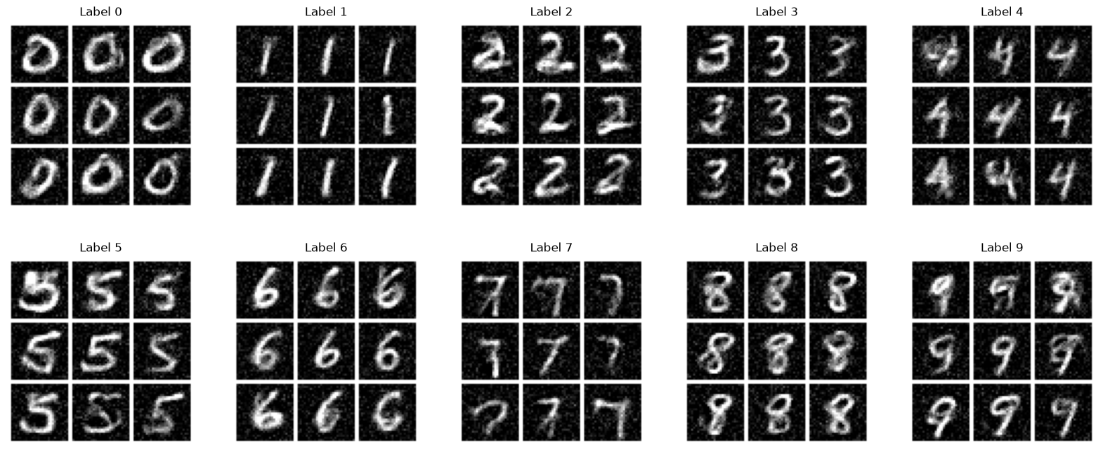
The tradeoff is that the class information is baked into the sampling procedure rather than the model, which makes it less flexible: you can’t easily interpolate between classes or use classifier-free guidance. But it’s a clean and surprisingly effective trick.

---

What’s Next

Part 2 will go further: flow inversion (running the ODE backwards to encode real images into noise), mode identification with multimodal source distributions, and time embeddings as an alternative to passing $t$ as a raw scalar. More on that when the experiments are done.